Code
library(tidyverse)
library(ggplot2)

knitr::opts_chunk$set(echo = TRUE, warning=FALSE, message=FALSE)library(tidyverse)
library(ggplot2)
knitr::opts_chunk$set(echo = TRUE, warning=FALSE, message=FALSE)Read Fedral Funds Rate data. I changed column names and added date column to make analyse easy.
ffr<-read_csv("_data/FedFundsRate.csv",
              show_col_types = FALSE,
              col_names = c("year","month","day","federal_funds_target_rate", "federal_funds_upper_target", "federal_funds_lower_target","effective_federal_funds_rate", "real_gdp", "unemployment_rate","inflation_rate"),
              skip=1)

library(lubridate)

ffr <- mutate(ffr, date = make_datetime(year, month, day))

ffr
# A tibble: 904 × 11
year month day federal_f…¹ feder…² feder…³ effec…⁴ real_…⁵ unemp…⁶ infla…⁷
<dbl> <dbl> <dbl> <dbl> <dbl> <dbl> <dbl> <dbl> <dbl> <dbl>
1 1954 7 1 NA NA NA 0.8 4.6 5.8 NA
2 1954 8 1 NA NA NA 1.22 NA 6 NA
3 1954 9 1 NA NA NA 1.06 NA 6.1 NA
4 1954 10 1 NA NA NA 0.85 8 5.7 NA
5 1954 11 1 NA NA NA 0.83 NA 5.3 NA
6 1954 12 1 NA NA NA 1.28 NA 5 NA
7 1955 1 1 NA NA NA 1.39 11.9 4.9 NA
8 1955 2 1 NA NA NA 1.29 NA 4.7 NA
9 1955 3 1 NA NA NA 1.35 NA 4.6 NA
10 1955 4 1 NA NA NA 1.43 6.7 4.7 NA
# … with 894 more rows, 1 more variable: date <dttm>, and abbreviated variable
# names ¹federal_funds_target_rate, ²federal_funds_upper_target,
# ³federal_funds_lower_target, ⁴effective_federal_funds_rate, ⁵real_gdp,
# ⁶unemployment_rate, ⁷inflation_rate
# ℹ Use `print(n = ...)` to see more rows, and `colnames()` to see all variable namescolnames(ffr) [1] "year" "month"
[3] "day" "federal_funds_target_rate"
[5] "federal_funds_upper_target" "federal_funds_lower_target"
[7] "effective_federal_funds_rate" "real_gdp"
[9] "unemployment_rate" "inflation_rate"
[11] "date" I’d like to check the time series of Real GDP and relation between Real GDP and Unemployment Rate after 2000. So I filtered after 2000 then selected Real GDP column and Unemployment column.
ffr2<-filter(ffr, year>=2000)
ffr2<-select(ffr2, year, real_gdp, unemployment_rate, date)
ffr2
# A tibble: 252 × 4
year real_gdp unemployment_rate date
<dbl> <dbl> <dbl> <dttm>
1 2000 1.2 4 2000-01-01 00:00:00
2 2000 NA 4.1 2000-02-01 00:00:00
3 2000 NA NA 2000-02-02 00:00:00
4 2000 NA 4 2000-03-01 00:00:00
5 2000 NA NA 2000-03-21 00:00:00
6 2000 7.8 3.8 2000-04-01 00:00:00
7 2000 NA 4 2000-05-01 00:00:00
8 2000 NA NA 2000-05-16 00:00:00
9 2000 NA 4 2000-06-01 00:00:00
10 2000 0.5 4 2000-07-01 00:00:00
# … with 242 more rows
# ℹ Use `print(n = ...)` to see more rowsTo make time series line graph, I removed the rows that has NA.
ffr2<-filter(ffr2, !is.na(real_gdp))
ffr2
# A tibble: 68 × 4
year real_gdp unemployment_rate date
<dbl> <dbl> <dbl> <dttm>
1 2000 1.2 4 2000-01-01 00:00:00
2 2000 7.8 3.8 2000-04-01 00:00:00
3 2000 0.5 4 2000-07-01 00:00:00
4 2000 2.3 3.9 2000-10-01 00:00:00
5 2001 -1.1 4.2 2001-01-01 00:00:00
6 2001 2.1 4.4 2001-04-01 00:00:00
7 2001 -1.3 4.6 2001-07-01 00:00:00
8 2001 1.1 5.3 2001-10-01 00:00:00
9 2002 3.7 5.7 2002-01-01 00:00:00
10 2002 2.2 5.9 2002-04-01 00:00:00
# … with 58 more rows
# ℹ Use `print(n = ...)` to see more rowsThen I drawed time line graph of real gdp.
ggplot(ffr2, aes(x=date, y=real_gdp)) +
  geom_line()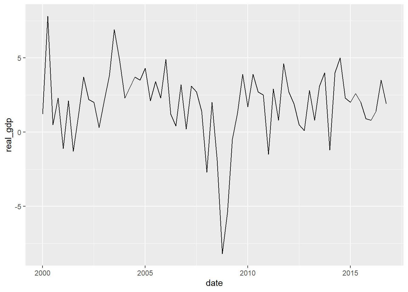
The line is usually between zero and five points during the period, but it hit a low during the financial crisis in the late 2000s.
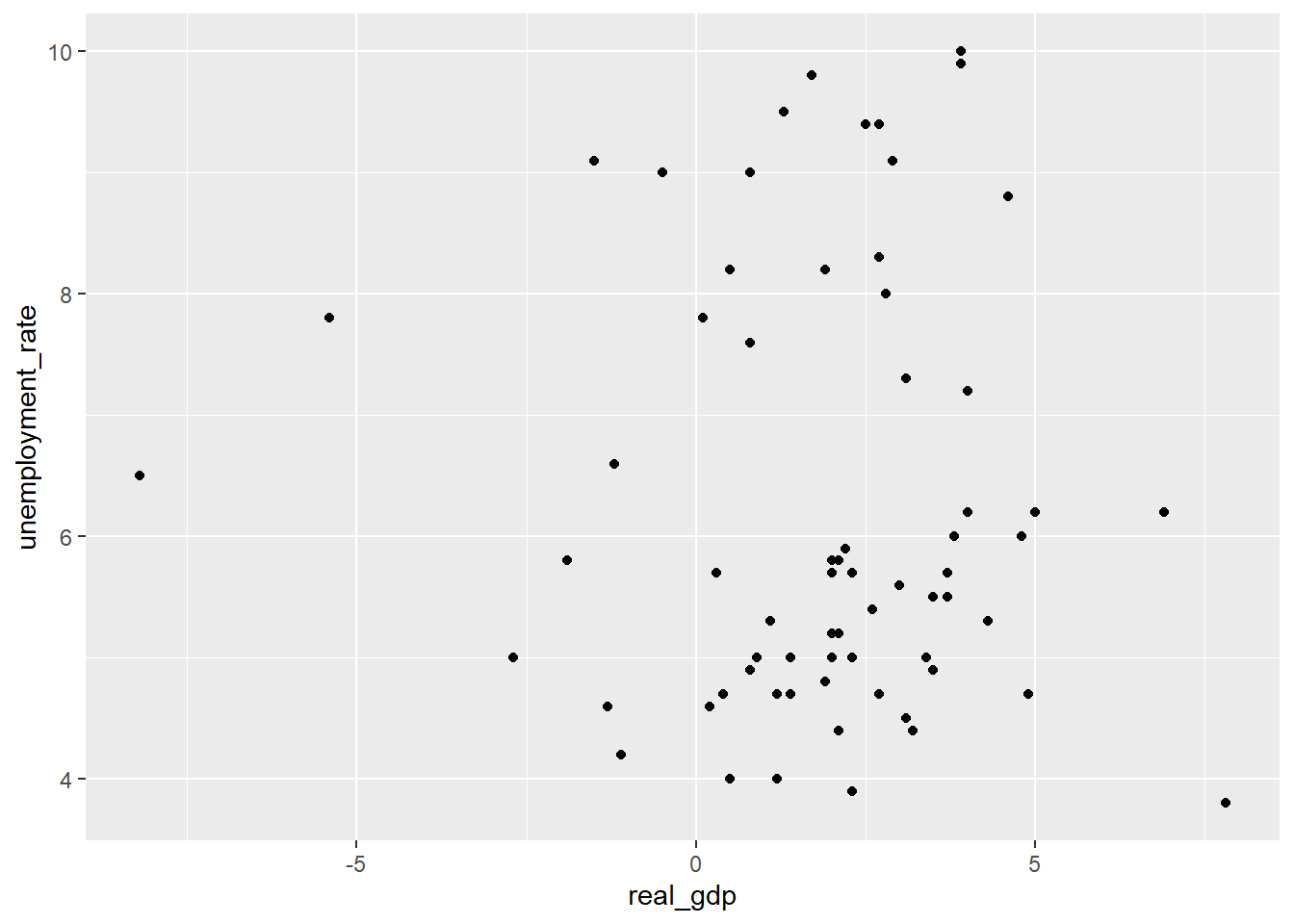
What I concerned is that the relation of real gdp growth and umemployment rate. So I drawed scatter plot of two variable. But according to the scatter plot, it looks like there are no clear relation between those two.
ggplot(ffr2, aes(x=real_gdp, y=unemployment_rate))+
  geom_point()